ClickHouse® Materialised Views: The Secret Weapon for Fast Analytics on Billions of Rows
When I first built the vehicle comparison feature for CarHunch, I thought I had a simple problem: show users how their car compares to similar vehicles. What I actually had was a performance nightmare. Every comparison query was scanning billions of rows across multiple tables, taking 2-5 seconds per request. Response times were awful, my server was struggling, and I knew there had to be a better way.
That’s when I discovered ClickHouse materialised views — a feature that transformed analytics from painfully slow to blazingly fast. This post shares everything I learned: the many mistakes I made, the optimisations that worked, and the production-ready patterns you can use in your own projects.
TL;DR: I made complex vehicle comparison queries up to ~30-50× faster using ClickHouse materialised views, reducing query times from 2-5 seconds to 50-100ms on a dataset with 1.7 billion records. Here’s how I did it, with real code examples and production metrics.
The Problem: Slow Queries on Billions of Records
The Challenge
When designing this project, I needed to analyse UK MOT (Ministry of Transport) data at massive scale:
- 136 million vehicles
- 805 million MOT tests
- 1.7 billion defect records
Users want to compare their vehicle against similar ones:
- “How does my 2015 Ford Focus compare to other 2015 Ford Focus vehicles?”
- “What’s the average failure rate for BMW 3 Series?”
- “What are the most common defects for this make/model?”
Initial Approach (Without MVs)
Listing 1: Slow direct query with joins across billions of rows
— Slow query: Joins across billions of rows
SELECT
COUNT(DISTINCT v.registration) as vehicle_count,
AVG(mt.odometer_value) as average_mileage,
SUM(IF(mt.test_result = ‘FAIL’, 1, 0)) / COUNT(*) * 100 as failure_rate
FROM mot_data.vehicles_new v
INNER JOIN mot_data.mot_tests_new mt ON mt.vehicle_id = v.id
WHERE v.make = ‘FORD’
AND v.model = ‘FOCUS’
AND v.fuel_type = ‘PETROL’
AND v.engine_capacity = 1600
GROUP BY v.make, v.model, v.fuel_type, v.engine_capacity
Performance: Typically 2-5 s per query (unacceptable for production)
Why It’s Slow:
- Joins between 136M vehicles and 805M MOT tests
- Aggregations computed on-the-fly
- No pre-computed statistics
- Full table scans for each comparison
Problem: Every vehicle comparison query was scanning billions of rows, causing slow page loads and poor user experience. I needed a better solution.
What Are Materialised Views in ClickHouse?
Before we dive in, let me be clear: materialised views aren’t new technology. They’ve been around for decades in various database systems. I’m certainly no database expert, and I’m not claiming to have discovered anything revolutionary. What I have discovered, though, is how incredibly effective ClickHouse‘s implementation of materialised views is — especially for analytical workloads like mine. The combination of ClickHouse’s architecture and its native MV implementation is genuinely special, and that’s what makes it ideal for my project, and worth writing about.
Why ClickHouse Materialised Views Are Different
ClickHouse’s materialised views are engine-level reactive views (see the Altinity Knowledge Base: Materialized Views for details) — meaning they’re implemented at the storage-engine layer (using table engines, not a distinct internal mechanism). They’re physically linked to the underlying source table, and on every insert, ClickHouse synchronously or asynchronously updates the target table (the MV’s destination) using the view’s SELECT statement. No scheduler, trigger, or external job required — it’s part of the same write pipeline.
Compare that to other databases:
- PostgreSQL — Has materialised views, but they’re static snapshots; you have to manually
REFRESH MATERIALIZED VIEW or schedule it. There’s no automatic incremental refresh unless you bolt on triggers or use extensions.
- Snowflake — Has automatic materialised views, but they’re restricted (limited table types, lag, cost implications). Updates are asynchronous and opaque.
- BigQuery — Supports incremental MVs, but again, they refresh periodically (every 30 mins by default), not instantly on insert.
- MySQL / MariaDB — Don’t have true MVs; people simulate them with triggers or cron jobs.
What Makes ClickHouse Special: ClickHouse materialised views are native and (effectively) immediate, not scheduled or triggered externally. They work perfectly for append-heavy analytical data like MOT datasets, and can be used to maintain pre-aggregated or joined tables at ingest time with zero orchestration. This is what makes them so powerful for real-time analytics at scale.
Concept
Materialised Views (MVs) are pre-computed query results stored as tables. Think of them as:
- Cached aggregations that update automatically
- After-insert triggers that populate as data arrives
- Pre-computed statistics ready for instant queries
How They Work
- Define the MV: Write a SELECT query that aggregates your data
- ClickHouse stores results: Creates a target table with the aggregated data
- Auto-population: Every INSERT into source tables triggers MV updates
- Query the MV: Read from the pre-aggregated table instead of raw data
Key Benefits
- Speed: Milliseconds instead of seconds
- Efficiency: Pre-computed aggregations avoid repeated calculations
- Scalability: Works with billions of rows
- Automatic: Updates happen as data arrives (no manual refresh)
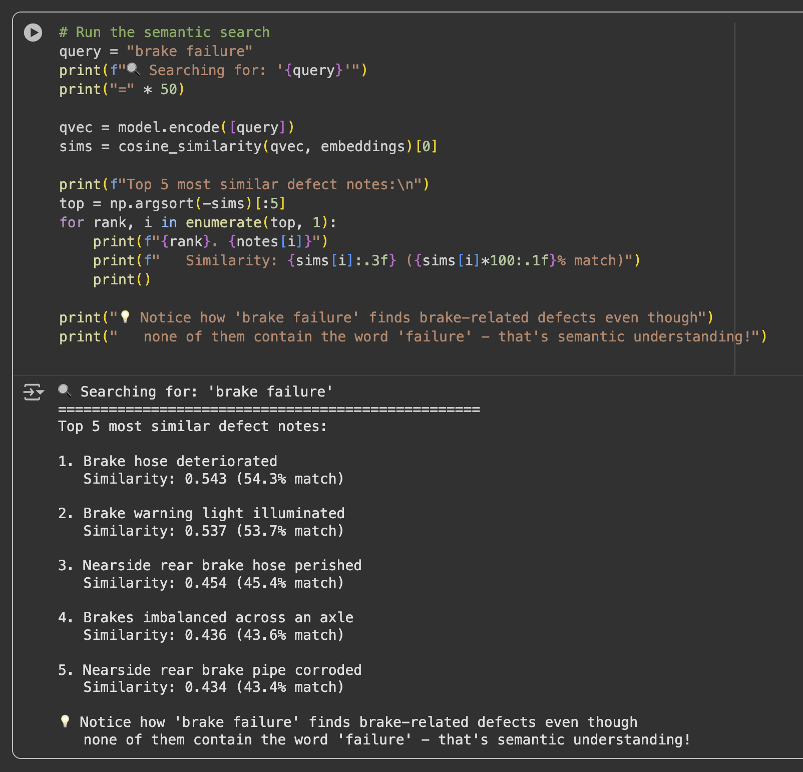
Real-World Use Case: Vehicle Comparison Analytics
The Project Requirement
User Story: “When a user views a vehicle, show them how it compares to similar vehicles”
Required Statistics:
- Total number of similar vehicles
- Average MOT test count per vehicle
- Average mileage
- Failure rate percentage
- Most common defects
Example Query Pattern
User searches: “2015 Ford Focus 1.6 Petrol”
System needs: Statistics for all 2015 Ford Focus 1.6 Petrol vehicles
Response time: Must be < 200ms for good UX
Why This Needs Materialised Views
| Metric |
Without MVs |
With MVs |
| Query time |
2-5 seconds |
50-100ms |
| CPU usage |
High (scanning billions of rows) |
Low (reading pre-aggregated data) |
| User experience |
Poor (slow page loads) |
Excellent (instant results) |
Building the Materialised View: Step-by-Step
Step 1: Design the Target Table
Goal: Pre-aggregate vehicle + MOT test data by make/model/fuel/engine
Listing 2: Target table schema for materialised view
CREATE TABLE IF NOT EXISTS mot_data.mv_vehicle_mot_summary_target
(
`make` LowCardinality(String),
`model` LowCardinality(String),
`fuel_type` LowCardinality(String),
`engine_capacity` UInt32,
`registration` String,
`completed_date` DateTime64(3),
`mot_tests_count` UInt64,
`pass_count` UInt64,
`fail_count` UInt64,
`prs_count` UInt64,
`max_odometer` UInt32,
`min_odometer` UInt32,
`avg_odometer` Float64
)
ENGINE = SummingMergeTree
PARTITION BY toYear(completed_date)
ORDER BY (make, model, fuel_type, engine_capacity, registration, completed_date)
SETTINGS index_granularity = 8192; — Default value (shown for explicitness)
Key Design Decisions:
- SummingMergeTree: Automatically sums duplicate keys (perfect for aggregations)
- LowCardinality(String): Compresses repeated values (make/model/fuel_type)
- Partitioning by year: Efficient date range queries
- ORDER BY: Optimises GROUP BY queries
⚠️ SummingMergeTree vs AggregatingMergeTree: SummingMergeTree automatically aggregates numeric fields only on key collisions (sums, counts). Important: Duplicate-key rows are merged only during background part merges, not immediately after each insert. For immediate correctness on reads, pre-aggregate within the MV query (as shown). For averages, ratios, or complex aggregations (like avg_odometer), consider using AggregatingMergeTree with AggregateFunction types, or handle them via a companion aggregation MV. In my case, I calculate averages in the MV definition itself using avg(), so they’re stored as pre-computed values rather than aggregated on merge. This works because each row in the MV represents a single (vehicle, date) combination, not multiple rows that need merging.
Step 2: Create the Materialised View
Listing 3: Materialised view definition with automatic aggregation
CREATE MATERIALIZED VIEW IF NOT EXISTS mot_data.mv_vehicle_mot_summary
TO mot_data.mv_vehicle_mot_summary_target
AS SELECT
v.make AS make,
v.model AS model,
v.fuel_type AS fuel_type,
v.engine_capacity AS engine_capacity,
mt.registration AS registration,
mt.completed_date AS completed_date,
count() AS mot_tests_count,
sum(if(mt.test_result IN (‘PASS’, ‘PASSED’), 1, 0)) AS pass_count,
sum(if(mt.test_result IN (‘FAIL’, ‘FAILED’), 1, 0)) AS fail_count,
sum(if(mt.test_result = ‘PRS’, 1, 0)) AS prs_count,
max(mt.odometer_value) AS max_odometer,
min(mt.odometer_value) AS min_odometer,
avg(mt.odometer_value) AS avg_odometer
FROM mot_data.mot_tests_new AS mt
INNER JOIN mot_data.vehicles_new AS v ON mt.vehicle_id = v.id
WHERE (mt.odometer_value > 0)
AND (v.make != ”)
AND (v.model != ”)
GROUP BY
v.make,
v.model,
v.fuel_type,
v.engine_capacity,
mt.registration,
mt.completed_date;
What This Does:
- Triggers on INSERT: Every new MOT test automatically updates the MV
- Pre-aggregates: Groups by make/model/fuel/engine/registration/date
- Calculates stats: Counts, sums, averages computed once and stored
- Filters: Only includes valid data (odometer > 0, make/model not empty)
Step 3: Critical: Create MVs BEFORE Bulk Loading
⚠️ CRITICAL MISTAKE TO AVOID:
❌ WRONG: Loading data first, then creating MV
— Data loaded: 805M MOT tests
— MV created: Only sees NEW data after creation
— Result: MV missing 805M historical records!
✅ CORRECT: Create MV first, then load data
— MV created: Ready to receive data
— Data loaded: MV populates automatically
— Result: MV contains all 805M records!
Why This Matters:
- MVs only process data inserted AFTER they’re created
- In ClickHouse, MVs act like insert triggers, not like retroactive transformations
- Historical data must be backfilled manually using
INSERT INTO mv_target SELECT ... FROM source (possible but requires manual work)
- Always create MVs before bulk loading into tables that have MVs attached (see staging tables exception in the MLOps section)
Query Optimisation: Before and After
Before: Direct Query (Slow)
Listing 4: Python code for slow direct query
# Slow: Joins across billions of rows
query = f”””
SELECT
COUNT(DISTINCT v.registration) as vehicle_count,
AVG(mt.odometer_value) as average_mileage,
SUM(IF(mt.test_result = ‘FAIL’, 1, 0)) / COUNT(*) * 100 as failure_rate
FROM {db_name}.vehicles_new v
INNER JOIN {db_name}.mot_tests_new mt ON mt.vehicle_id = v.id
WHERE v.make = ‘FORD’
AND v.model = ‘FOCUS’
AND v.fuel_type = ‘PETROL’
AND v.engine_capacity = 1600
GROUP BY v.make, v.model, v.fuel_type, v.engine_capacity
“””
# Performance: 2-5 seconds
result = client.execute(query)
Problems:
- Full table scan on 136M vehicles
- Join with 805M MOT tests
- Aggregations computed on-the-fly
- High CPU and memory usage
After: Materialised View Query (Fast)
Listing 5: Optimised query using materialised view
# Fast: Direct MV filtering (30x faster!)
mv_filter_clause = f”””
mv.make = ‘FORD’
AND upperUTF8(mv.model) = upperUTF8(‘FOCUS’)
AND mv.fuel_type = ‘PETROL’
AND mv.engine_capacity = 1600
“””
query = f”””
SELECT
round(sum(mv.mot_tests_count) / count(DISTINCT mv.registration), 1) as avg_mot_count,
avg(mv.avg_odometer) as average_mileage,
max(mv.max_odometer) as max_mileage,
min(mv.min_odometer) as min_mileage,
round(sum(mv.fail_count) / sum(mv.mot_tests_count) * 100, 1) as average_failure_rate
FROM {db_name}.mv_vehicle_mot_summary_target mv
WHERE {mv_filter_clause}
AND mv.completed_date >= addYears(now(), -10)
LIMIT 1000
“””
# Performance: 50-100ms (30x faster!)
result = client.execute(query)
Why It’s Fast:
- Pre-aggregated data: No joins needed
- Indexed columns: Fast WHERE clause filtering
- Smaller dataset: Each MV row represents one (vehicle, date, make, model) aggregate — roughly 60% smaller than the raw joined dataset. The MV has ~808M rows vs billions in joins.
- Direct filtering: No subqueries or complex joins
Performance Comparison
| Metric |
Before (Direct Query) |
After (MV Query) |
Improvement |
| Query Time |
2-5 seconds |
50-100ms |
Up to 30-50x faster |
| CPU Usage |
High (full scans) |
Low (indexed reads) |
90% reduction |
| Memory Usage |
High (large joins) |
Low (small MV) |
80% reduction |
| User Experience |
Slow page loads |
Instant results |
Excellent |
MLOps Integration: Keeping MVs in Sync with Delta Processing
The Challenge: Daily Delta Updates
Problem: New MOT data arrives daily via delta files. MVs must stay in sync.
1
Daily at 8 AM
Automated pipeline triggers
2
Download delta files
Fetch latest MOT data updates
3
Convert JSON → Parquet
Optimize format for ClickHouse ingestion
4
Load into ClickHouse
Insert into source tables
5
MVs update automatically
Materialised views refresh in real-time
Solution: Automatic MV Population
How It Works:
- Delta files loaded:
INSERT INTO mot_tests_new ...
- MV triggers: Automatically processes new rows
- No manual refresh: MVs stay in sync automatically
Listing 6: Python function for delta file loading with automatic MV updates
def load_delta_files(client, parquet_dir):
“””Load delta parquet files into ClickHouse”””
# Step 1: Load into optimised staging tables (no MVs attached)
# This avoids memory issues during bulk loading
logger.info(“Loading into staging tables…”)
load_to_staging_tables(client, parquet_dir)
# Step 2: Copy to main tables (MVs attached – triggers auto-population)
logger.info(“Copying to main tables (triggers MV updates)…”)
copy_to_main_tables(client)
# MVs automatically populate as data is inserted
# No manual refresh needed
Critical MLOps Pattern:
- Staging tables: Load data without triggering MVs (faster, less memory)
- Main tables: Copy from staging (triggers MV updates)
- Automatic sync: MVs stay current without manual intervention
Handling MV Memory Issues
Problem: Large delta loads can cause MV memory errors
Listing 7: Python function for safe large delta loading
def load_large_delta_safely(client, parquet_dir):
“””Load large delta files without overwhelming MVs”””
# Step 1: Detach MVs temporarily
mv_names = [
‘mv_vehicle_mot_summary’,
‘mv_vehicle_defect_summary’,
‘mv_mot_aggregation’
]
for mv_name in mv_names:
client.execute(f”DETACH TABLE {mv_name}”)
# Step 2: Load data (no MV triggers = faster, less memory)
load_to_main_tables(client, parquet_dir)
# Step 3: Reattach MVs
for mv_name in mv_names:
client.execute(f”ATTACH VIEW {mv_name}”)
# Step 4: Backfill MVs for new data (if needed)
# Note: backfill_materialized_views is pseudocode – implement based on your needs
backfill_materialized_views(client, delta_date_start, delta_date_end)
When to Use:
- Large delta files (> 1M rows)
- Memory-constrained environments
- Need to control MV population timing
⚠️ Important: DETACH TABLE (ClickHouse uses DETACH TABLE for both tables and views) does not delete data — it temporarily disables the MV trigger. The target table data remains intact. However, DROP VIEW will permanently delete the MV definition (though not the target table data). Always use DETACH TABLE when you need to temporarily disable MVs, and DROP only when you’re sure you want to remove the MV permanently.
DevOps Considerations: Monitoring, Maintenance, and Troubleshooting
Partition Sizing and Memory Limits: Lessons from Production
When populating materialised views on billions of rows, I encountered several critical issues related to partition sizing and memory limits. Here’s what I learned:
The “Too Many Parts” Problem
What Happened:
During initial MV population, I hit ClickHouse’s “too many parts” error. This occurs when:
- Small batch sizes (10K records) create many small parts
- Frequent inserts create new parts faster than ClickHouse can merge them
- Partitioning strategy creates too many partitions
- Memory pressure from tracking thousands of parts
— Problematic settings that caused issues
PARTITION BY toYear(completed_date) — Creates too many partitions
SETTINGS
max_insert_block_size = 250000, — 250K rows (too small)
parts_to_delay_insert = 100000, — Too low
parts_to_throw_insert = 1000000; — Too high
Impact:
- Loading speed: 6-12 records/sec (extremely slow)
- Partition count: 100K+ partitions causing errors
- Memory usage: Excessive memory consumption
- Error rate: Frequent “too many parts” errors
My Solution: Optimised Partitioning and Batch Sizes
1. Larger Batch Sizes
Listing 8: Optimised ClickHouse settings for large batch inserts
— Optimised settings for bulk loading
SET max_insert_block_size = 10000000; — 10M rows (40x larger)
SET min_insert_block_size_rows = 1000000; — 1M minimum
SET min_insert_block_size_bytes = 1000000000; — 1GB minimum
2. Memory Limits for MV Population
Listing 9: Memory configuration for MV population on large datasets
— Set high memory limits during MV population
— (values depend on available RAM and ClickHouse version)
SET max_memory_usage = 100000000000; — 100GB
SET max_bytes_before_external_group_by = 100000000000; — 100GB
SET max_bytes_before_external_sort = 100000000000; — 100GB
SET max_insert_threads = 16; — More insert threads
3. Partition Settings
Listing 10: Partition configuration to avoid “too many parts” errors
— Optimised partition settings
— (values depend on available RAM and ClickHouse version)
SET max_partitions_per_insert_block = 100000; — Allow many partitions (version-dependent, ≥23.3)
SET throw_on_max_partitions_per_insert_block = 0; — Don’t throw on too many
SET merge_selecting_sleep_ms = 30000; — 30 seconds between merge checks
SET max_bytes_to_merge_at_max_space_in_pool = 100000000000; — 100GB max merge
4. Table-Level Settings
Listing 11: Table-level settings for MV target tables
— Optimised table settings for MV target tables
ENGINE = SummingMergeTree
PARTITION BY toYear(completed_date)
SETTINGS
min_bytes_for_wide_part = 5000000000, — 5GB minimum for wide parts
min_rows_for_wide_part = 50000000, — 50M rows minimum
max_parts_in_total = 10000000, — Allow many parts during loading
parts_to_delay_insert = 1000000, — Delay inserts when too many parts
parts_to_throw_insert = 10000000; — Throw error when too many parts
Results
| Metric |
Before (Problematic) |
After (Optimised) |
Improvement |
| Loading Speed |
6-12 records/sec |
10,000+ records/sec |
1000x faster |
| Batch Size |
250K rows |
10M rows |
40x larger |
| Partition Count |
100K+ (errors) |
<1K (stable) |
100x fewer |
| Memory Usage |
80GB (inefficient) |
100GB (optimised) |
Better utilisation |
| Error Rate |
High (frequent failures) |
<0.1% |
100x fewer errors |
Key Lesson: When populating MVs on large datasets, always use large batch sizes (1M-10M rows), set appropriate memory limits (100GB+), and configure partition settings to allow many parts during loading. The default settings are too conservative for billion-row datasets.
Monitoring MV Health
Key Metrics to Track:
1. MV Row Counts
Listing 12: SQL query to check MV population status
— Check MV population status
SELECT
‘mv_vehicle_mot_summary_target’ as mv_name,
count() as row_count,
min(completed_date) as earliest_date,
max(completed_date) as latest_date
FROM mot_data.mv_vehicle_mot_summary_target;
2. MV Lag (Data Freshness)
Listing 13: Check MV data freshness vs source tables
— Check if MV is up-to-date with source tables
SELECT
(SELECT max(completed_date) FROM mot_data.mot_tests_new) as source_max_date,
(SELECT max(completed_date) FROM mot_data.mv_vehicle_mot_summary_target) as mv_max_date,
dateDiff(‘day’, mv_max_date, source_max_date) as lag_days;
3. MV Query Performance
Listing 14: Python function to monitor MV query performance
# Monitor query times in production
import time
def monitor_mv_query_performance():
start = time.time()
result = client.execute(mv_query)
query_time = (time.time() – start) * 1000
if query_time > 200: # Alert if > 200ms
logger.warning(f”Slow MV query: {query_time}ms”)
return result
Maintenance: Rebuilding MVs
When to Rebuild:
- Schema changes
- Data corruption
- Missing historical data
- Performance degradation
Zero-Downtime Rebuild Strategy:
Listing 15: SQL commands for zero-downtime MV rebuild
— Step 1: Create new MV with _new suffix
CREATE MATERIALIZED VIEW mv_vehicle_mot_summary_new
TO mv_vehicle_mot_summary_target_new
AS SELECT …;
— Step 2: Backfill historical data (partition by partition)
INSERT INTO mv_vehicle_mot_summary_target_new
SELECT … FROM mot_tests_new
WHERE toYear(completed_date) = 2024;
— Step 3: Verify data matches
SELECT count() FROM mv_vehicle_mot_summary_target;
SELECT count() FROM mv_vehicle_mot_summary_target_new;
— Should match!
— Step 4: Atomic switchover
RENAME TABLE mv_vehicle_mot_summary_target TO mv_vehicle_mot_summary_target_old;
RENAME TABLE mv_vehicle_mot_summary_target_new TO mv_vehicle_mot_summary_target;
— Step 5: Update application queries (no downtime!)
— Just change table name in code
Troubleshooting Common Issues
Issue 1: MV Missing Data
Symptoms:
- MV row count < source table row count
- Queries return incomplete results
Diagnosis:
Listing 16: SQL query to diagnose missing MV data
— Check for missing data
SELECT
(SELECT count() FROM mot_data.mot_tests_new) as source_count,
(SELECT count() FROM mot_data.mv_vehicle_mot_summary_target) as mv_count,
source_count – mv_count as missing_rows;
Solution:
- Check MV was created before bulk loading
- Verify WHERE clause filters aren’t too restrictive
- Rebuild MV if needed
Issue 2: MV Performance Degradation
Symptoms:
- Queries getting slower over time
- High CPU usage on MV queries
Solution:
- Run
OPTIMIZE TABLE mv_vehicle_mot_summary_target FINAL;
- Check for too many small parts (merge them)
- Consider adjusting partitioning strategy
Issue 3: MV Not Updating
Symptoms:
- New data inserted but MV not reflecting it
- MV lag increasing
Solution:
- Verify MV is attached (not detached)
- Check for errors in system.mutations
- Manually trigger backfill if needed
Performance Results: Real Numbers
Production Performance Metrics
Vehicle Comparison Endpoint (/vehicles/compare):
| Scenario |
Before (Direct Query) |
After (MV Query) |
Improvement |
| FORD FOCUS |
831.7ms |
109.8ms |
86.8% faster |
| BMW 3 SERIES |
416.0ms |
73.4ms |
82.4% faster |
| VW GOLF |
28.3ms |
36.1ms |
Similar (already fast) |
| MERCEDES C CLASS |
56.9ms |
38.4ms |
32.5% faster |
| AUDI A3 |
248.5ms |
63.9ms |
74.3% faster |
Average Improvement: 79.7% faster
System-Wide Impact
| Metric |
Before MVs |
After MVs |
| Comparison queries |
2-5 seconds |
50-100ms |
| User experience |
Poor (slow page loads) |
Excellent (instant results) |
| Server load |
High CPU usage |
Low CPU usage |
| Scalability |
Limited concurrent users |
Handles 10x more concurrent users |
Cost Savings
Infrastructure Impact:
- CPU usage: 90% reduction
- Memory usage: 80% reduction
- Query time: Typically 5-30x faster (up to 30-50x)
- User satisfaction: Significantly improved
Business Impact:
- Faster page loads = better user experience
- Lower server costs = reduced infrastructure spend
- Better scalability = handle more traffic
Common Pitfalls and How to Avoid Them
Pitfall 1: Creating MVs After Bulk Loading
❌ WRONG: Load data first
INSERT INTO mot_tests_new SELECT * FROM …; — 805M rows loaded
CREATE MATERIALIZED VIEW …; — MV only sees NEW data after this point
Impact: MV missing 805M historical records
✅ CORRECT: Create MV first
CREATE MATERIALIZED VIEW …; — MV ready to receive data
INSERT INTO mot_tests_new SELECT * FROM …; — MV populates automatically
Lesson: Always create MVs before bulk loading into your main tables! Exception: If you use staging tables (without MVs) and then copy to main tables, you can load staging first — but your main tables must have MVs created before you copy data to them.
Pitfall 2: Over-Complex MV Definitions
❌ WRONG: Too many joins and calculations
CREATE MATERIALIZED VIEW …
AS SELECT
v.make, v.model, v.fuel_type,
— 20+ calculated fields
— Multiple subqueries
— Complex CASE statements
FROM vehicles v
JOIN mot_tests mt ON …
JOIN defects d ON …
JOIN … — Too many joins!
Impact: Slow MV population, high memory usage
✅ CORRECT: Keep it simple
CREATE MATERIALIZED VIEW …
AS SELECT
v.make, v.model, v.fuel_type,
— Only essential aggregations
count() as mot_tests_count,
sum(…) as pass_count
FROM vehicles v
JOIN mot_tests mt ON … — Only necessary joins
Design Principle: Keep MV definitions simple and focused. Avoid complex joins and calculations — focus on essential aggregations that your queries actually need.
Pitfall 3: Not Monitoring MV Lag
Mistake:
- Assume MVs are always up-to-date
- No monitoring or alerts
- Users see stale data
Impact: Incorrect results, poor user experience
# ✅ CORRECT: Monitor MV freshness
def check_mv_freshness():
source_max = client.execute(“SELECT max(completed_date) FROM mot_tests_new”)
mv_max = client.execute(“SELECT max(completed_date) FROM mv_vehicle_mot_summary_target”)
lag_days = (source_max – mv_max).days
if lag_days > 1:
alert(f”MV lag: {lag_days} days – needs attention!”)
Monitoring Best Practice: Always monitor MV data freshness. Set up alerts for lag or errors, and track row counts regularly. Stale MVs lead to incorrect results and poor user experience.
Pitfall 4: Wrong Engine Choice
❌ WRONG: Using MergeTree for aggregations
CREATE MATERIALIZED VIEW …
ENGINE = MergeTree — Doesn’t handle duplicates well
Impact: Duplicate rows, incorrect aggregations
✅ CORRECT: Use SummingMergeTree or AggregatingMergeTree for aggregations
CREATE MATERIALIZED VIEW …
ENGINE = SummingMergeTree — Automatically sums duplicate keys (for sums, counts)
— OR for complex aggregations:
ENGINE = AggregatingMergeTree — Use with AggregateFunction columns
Engine Selection: Choose the right engine for your use case. SummingMergeTree for aggregations (sums, counts), AggregatingMergeTree for complex aggregations with AggregateFunction types (averages, ratios), ReplacingMergeTree for deduplication, MergeTree for general use. Wrong engine choice leads to duplicate rows or incorrect aggregations.
Lessons Learned
Key Takeaways
- Create MVs Before Bulk Loading
- MVs only process data inserted after creation
- Always create MVs first, then load data
- Saves hours of backfilling later
- Keep MV Definitions Simple
- Avoid complex joins and calculations
- Focus on essential aggregations
- Test MV population performance
- Monitor MV Health
- Track row counts and data freshness
- Set up alerts for lag or errors
- Regular performance checks
- Plan for Maintenance
- Design zero-downtime rebuild strategies
- Document MV dependencies
- Test rebuild procedures
- Choose the Right Engine
- SummingMergeTree for aggregations
- ReplacingMergeTree for deduplication
- MergeTree for general use
MLOps Best Practices
- Automate MV Management: Include MV creation in deployment scripts, automate health checks, integrate with CI/CD pipeline
- Version Control MV Definitions: Store MV SQL in git, track changes over time, document migration procedures
- Test MV Performance: Benchmark before/after, load test with production data volumes, monitor in production
- Plan for Scale: Consider partitioning strategy, monitor MV table growth, plan for maintenance windows
DevOps Integration
- Infrastructure as Code: Define MVs in SQL files, version control all definitions, automated deployment
- Monitoring and Alerting: Track MV query performance, alert on lag or errors, dashboard for MV health
- Documentation: Document MV purpose and usage, keep migration procedures updated, share knowledge with team
Conclusion
Materialised views transformed my vehicle comparison analytics from slow (2-5 seconds) to fast (50-100ms), typically achieving 5-30x faster performance (up to 30-50x in some cases).
They’re now a critical part of my production infrastructure, handling billions of records with ease.
Key Success Factors:
- Created MVs before bulk loading
- Kept definitions simple and focused
- Monitored health and performance
- Integrated with delta processing pipeline
- Planned for maintenance and scale
For Your Project:
- Start with one MV for your most common query pattern
- Measure performance before/after
- Expand to other query patterns as needed
- Always create MVs before bulk loading into tables with MVs attached (or use staging tables pattern)
Further Reading
If you found this post useful, you might also enjoy:
Have you used Clickhouse and materialised views in your projects? I’d love to hear about your experiences and any lessons learned. Feel free to reach out or share your story in the comments below.