Advanced Risk Management for Freqtrade: Integrating Real-Time Market Awareness
Freqtrade is a popular open-source cryptocurrency trading bot framework. It gives you solid tools for strategy development, backtesting, and running automated trading strategies live – and it does a very good job of evaluating individual trade entries and exits.
I’ve used Freqtrade extensively, both for testing ideas and for running strategies live.
One thing I kept running into, though, was that while Freqtrade is very good at answering one question:
“Is this a valid entry signal right now?”
…it doesn’t really answer a different, higher-level one:
“Is this a market worth trading at all right now?”
If you’ve run Freqtrade strategies with real money, you’ve probably seen the same pattern: strategies that look perfectly reasonable in backtests, with sensible entry logic and risk controls, can still bleed during periods of high volatility, regime shifts, or market-wide panic – even when individual entries look fine in isolation.
That gap is what led me to experiment with a separate market-level risk layer, which eventually became Remora.
Rather than changing strategy logic or adding yet another indicator, Remora sits outside the strategy and provides a market-level risk assessment – answering whether current conditions are historically safe or risky to trade, regardless of what your entry signals are doing.
Importantly, this is an additive layer – your strategy logic and entry signals remain unchanged.
This article walks through how that works, how to integrate it into Freqtrade safely, and how to validate its impact using reproducible backtests.
TL;DR: This article shows how to add real-time market risk filtering to Freqtrade using Remora, a small standalone microservice that aggregates volatility, regime, sentiment, and macro signals. Integration is fail-safe, transparent, and requires only a minimal change to your strategy code.
What This Article Covers
- Why market regime risk matters for Freqtrade strategies
- What Remora does (at a high level)
- How to integrate it safely without breaking your strategy
- How to validate its impact using reproducible backtests
Who This Is For (And Who It Isn’t)
This is likely useful if you:
- Run live Freqtrade bots with real capital
- Care about drawdowns and regime risk, not just backtest curves
- Want a fail-safe, auditable risk layer
- Prefer transparent systems over black-box signals
This is probably not useful if you:
- Want a plug-and-play “buy/sell” signal
- Optimise single backtests rather than live behaviour
- Expect risk filters to magically fix bad strategies
Part 1: The Missing Layer in Most Freqtrade Strategies
Market conditions aren’t always tradable. Periods of extreme volatility, panic regimes, bear markets, and negative sentiment cascades can turn otherwise solid strategies into consistent losers – even when individual entries look fine in isolation.
Typical Freqtrade risk controls (position sizing, stop-losses, portfolio exposure) protect individual trades, but they don’t address market regime risk – the question of whether current market conditions are fundamentally safe to trade in at all.
Part 2: Remora – Market-Wide Risk as a Service
Remora is a standalone market-risk engine designed to sit outside your strategy logic.
Instead of changing how your strategy finds entries, Remora answers one question:
“Are current market conditions safe to trade?”
Results at a Glance (Why This Matters)
Before diving into implementation details, it’s useful to see what this approach looks like in practice.
Across 6 years of data (2020-2025), 4 different strategies, and 20 backtests:
- 90% of tests improved performance (18 out of 20)
- +1.54% average profit improvement
- +1.55% average drawdown reduction
- 4.3% of trades filtered (adaptive – increases to 16-19% during bear markets)
- Strongest impact during bear markets (2022 saw 16-19% filtering during crashes)
All results are fully reproducible using an open-source backtesting framework (details later).
Core Design Principles
- Fail-open by default: If Remora is unavailable, your bot continues trading normally.
- Transparent decisions: Every response includes human-readable reasoning.
- Multi-source aggregation: Dozens of signals with redundancy and failover.
- Low-latency: Designed for synchronous use inside live trading loops.
- No lock-in: Simple HTTP API. Remove it by deleting a few lines of code.
Data Aggregation Strategy (High-Level)
Rather than relying on a single indicator, Remora combines multiple signal classes:
Technical & Market Structure:
- Volatility metrics (realised, model-based)
- Momentum indicators
- Regime classification (bull / bear / choppy / panic)
- Volume and market structure signals
Sentiment & Macro:
- News sentiment (multi-source)
- Fear & Greed Index
- Funding rates and liquidations
- BTC dominance
- Macro correlations (e.g. VIX, DXY)
Each signal type has multiple providers. If one source fails or becomes stale, others continue supplying data.
The output is:
safe_to_trade (boolean)risk_score (0-1)- market regime
- volatility metrics
- clear textual reasoning
Part 3: Freqtrade Integration (Minimal & Reversible)
Integration uses Freqtrade’s confirm_trade_entry hook.
You do not modify your strategy’s entry logic – you simply gate entries at the final step.
Step-by-Step Integration
Here’s exactly what to add to your existing Freqtrade strategy. The code is color-coded: gray shows your existing code, green shows the new Remora integration code.
Step 0: Set Your API Key
Before running your strategy, set the environment variable:
export REMORA_API_KEY=”your-api-key-here”
Get your free API key at remora-ai.com/signup.php
Step 1: Add Remora to Your Strategy
Insert the green code blocks into your existing strategy file exactly as shown:
class MyStrategy(IStrategy):
    # ----- EXISTING STRATEGY LOGIC -----
    def populate_entry_trend(self, dataframe: DataFrame, metadata: dict) -> DataFrame:
        pair = metadata['pair']

        # Your existing entry conditions...
        # dataframe.loc[:, 'enter_long'] = 1  # example existing logic

        # ----- REMORA CHECK -----
        if not self.confirm_trade_entry(pair):
            dataframe.loc[:, 'enter_long'] = 0  # REMORA: Skip high-risk trades

        return dataframe

    # ----- ADD THIS NEW METHOD -----
    def confirm_trade_entry(self, pair: str, **kwargs) -> bool:
        import os
        import requests
        api_key = os.getenv("REMORA_API_KEY")
        headers = {"Authorization": f"Bearer {api_key}"} if api_key else {}

        try:
            r = requests.get(
                "https://remora-ai.com/api/v1/risk",
                params={"pair": pair},
                headers=headers,
                timeout=2.0
            )
            return r.json().get("safe_to_trade", True)  # REMORA: Block entry if market is high-risk
        except Exception:
            return True  # REMORA: Fail-open
Integration Notes:
- Inside your existing
populate_entry_trend(), insert the green Remora check just before return dataframe.
- After that, add the green
confirm_trade_entry() method at the same indentation level as your other strategy methods.
- All green comments are prefixed with
# REMORA: so you can easily identify or remove them later.
- Everything else in your strategy stays unchanged.
Removing Remora is as simple as deleting these lines. No lock-in, fully transparent.
Pair-Specific vs Market-Wide Risk
You can query Remora in two modes:
Pair-specific:
params={“pair”: “BTC/USDT”}
Market-wide (global trade gating):
# No pair parameter
Many users start with market-wide gating to reduce API calls and complexity.
What the API Returns
{
“safe_to_trade”: false,
“risk_score”: 0.75,
“regime”: “bear”,
“volatility”: 0.68,
“reasoning”: [
“High volatility detected”,
“Bear market regime identified”,
“Fear & Greed Index: Extreme Fear”,
“Negative news sentiment”
]
}
This allows debugging blocked trades, auditing decisions, custom logic layered on top, and strategy-specific thresholds.
Part 4: Backtesting & Validation (Reproducible)
Live APIs don’t work in historical backtests – so Remora includes an open-source backtesting framework that reconstructs historical risk signals using the same logic as production.
Repository: github.com/DonaldSimpson/remora-backtests
What It Provides
- Historical signal reconstruction
- Baseline vs Remora-filtered comparisons
- Multiple strategy types
- Consistent metrics and visualisations
What It Shows
- Improvements are not strategy-specific
- Filtering increases during crashes
- Small trade suppression can meaningfully reduce drawdowns
- Performance gains come from avoiding bad periods, not over-trading
You’re encouraged to run this yourself and independently verify the impact on your own strategies.
Here’s what comprehensive backtesting across 6 years (2020-2025), 4 different strategies, and 20 test cases has proven:
Overall Performance Improvements
| Metric |
Result |
| Average Profit Improvement |
+1.54% (18 out of 20 tests improved – 90% success rate) |
| Average Drawdown Reduction |
+1.55% (18 out of 20 tests improved) |
| Trades Filtered |
4.3% (2,239 out of 51,941 total trades) |
| Best Strategy Improvement |
+3.20% (BollingerBreakout strategy) |
| Most Effective Period |
2022 Bear Market (16-19% filtering during crashes) |
Financial Impact by Account Size
Based on average improvements, here’s the financial benefit on different account sizes:
| Account Size |
Additional Profit |
Reduced Losses |
Total Benefit |
| $10,000 |
+$154.25 |
+$154.70 |
$308.95 |
| $50,000 |
+$771.25 |
+$773.50 |
$1,544.75 |
| $100,000 |
+$1,542.50 |
+$1,547.00 |
$3,089.50 |
| $500,000 |
+$7,712.50 |
+$7,735.00 |
$15,447.50 |
| $1,000,000 |
+$15,425.00 |
+$15,470.00 |
$30,895.00 |
What These Numbers Mean
- 4.3% Trade Filtering: Remora prevents trades during dangerous market periods. This is adaptive – during the 2022 bear market, filtering increased to 16-19%, showing Remora becomes more protective when markets are most dangerous.
- +1.54% Profit Improvement: By avoiding bad trades during high-risk periods, strategies show consistent profit improvements. 90% of tests (18 out of 20) showed improvement.
- +1.55% Drawdown Reduction: Less maximum loss during unfavorable periods. This is critical for risk management and capital preservation.
- Best During Crashes: Remora is most effective during bear markets and crashes (2022 showed 16-19% filtering), exactly when you need protection most.
Part 5: Production & Advanced Use
Always fail-open:
except requests.Timeout:
return True
Log decisions:
logger.info(
f”Remora: safe={safe}, risk={risk_score}, regime={regime}”
)
Reduce API load:
- Cache responses (e.g. 30s)
- Use market-wide checks
- Upgrade tier only if needed
Advanced Uses (Optional)
- Dynamic position sizing based on risk_score
- Strategy-specific risk thresholds
- Regime-based strategy switching
- Trade blocking during macro stress events
These are additive – not required to get value.
Part 6: Technical Implementation Details
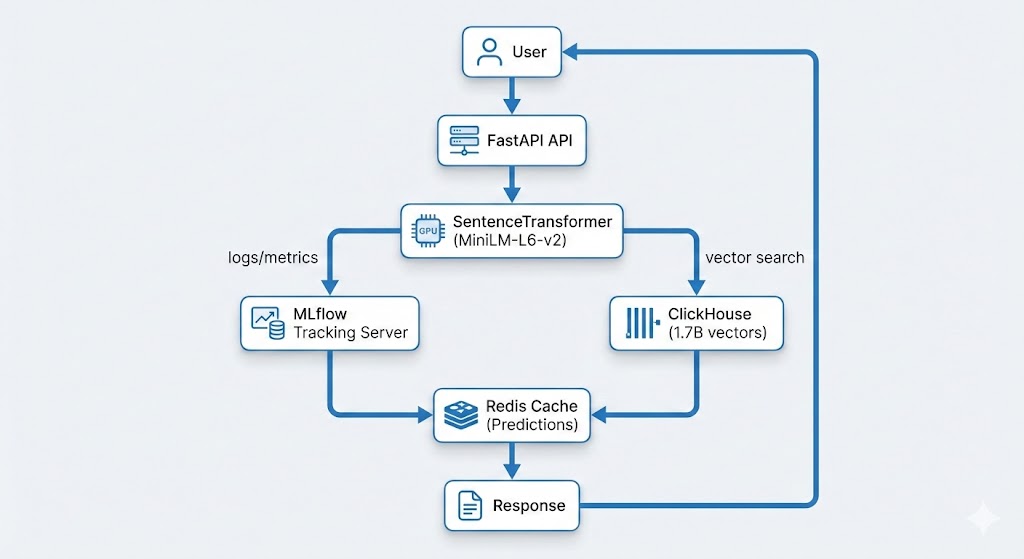
Data Pipeline Architecture
Remora’s data pipeline follows a producer-consumer pattern:
- Data Collection: Multiple scheduled tasks fetch data from various sources (Binance API, CoinGecko, news APIs, etc.)
- Data Storage: Raw data stored in ClickHouse time-series database
- Materialized Views: ClickHouse materialized views pre-aggregate data for fast queries
- Risk Calculation: Python service calculates risk scores using aggregated data
- Caching: Redis caches risk assessments to reduce database load
- API Layer: FastAPI serves risk assessments via REST API
ClickHouse Materialized Views
ClickHouse materialized views enable real-time aggregation without query-time computation overhead:
CREATE MATERIALIZED VIEW volatility_1h_mv
ENGINE = AggregatingMergeTree()
ORDER BY (pair, timestamp_hour)
AS SELECT
pair,
toStartOfHour(timestamp) as timestamp_hour,
avgState(price) as avg_price,
stddevSampState(price) as volatility
FROM raw_trades
GROUP BY pair, timestamp_hour;
This allows Remora to provide real-time risk assessments with minimal latency, even when processing millions of data points.
Failover & Redundancy
Each data source has multiple providers with automatic failover. This ensures reliable risk assessments even if individual data sources experience outages or rate limiting.
def get_fear_greed_index():
“””
Fetch Fear & Greed Index with multi-provider failover.
Tries multiple sources until one succeeds.
“””
providers = [
fetch_from_alternative_me,
fetch_from_coinmarketcap,
fetch_from_custom_source,
fetch_from_backup_provider_1,
fetch_from_backup_provider_2,
# … additional providers for redundancy
]
# Try each provider until one succeeds
for provider in providers:
try:
data = provider()
if data and is_valid(data):
return data
except Exception:
continue
# If all providers fail, return None
# The risk calculator handles missing data gracefully
return None
This multi-provider approach ensures:
- High Availability: If one provider fails, others continue providing data
- Rate Limit Resilience: Multiple providers mean you’re not dependent on a single API’s rate limits
- Data Quality: Can validate data across providers and choose the most reliable source
- Graceful Degradation: If all providers for one signal type fail, the risk calculator continues using other available signals (volatility, regime, sentiment, etc.)
In Remora’s implementation, each signal type (Fear & Greed, news sentiment, funding rates, etc.) has multiple providers. If one data source is unavailable, others continue providing information, ensuring the system maintains reliable risk assessments even during external API outages.
Security & Best Practices
- API Key Management: Store API keys in environment variables, never in code
- HTTPS Only: Always use HTTPS for API calls (Remora enforces this)
- Rate Limiting: Respect rate limits to avoid service disruption
- Monitoring: Monitor Remora API response times and error rates
- Fail-Open: Always implement fail-open behaviour – never let Remora block your entire trading system
API Access & Pricing
Remora offers a tiered API access structure designed to accommodate different use cases:
Unauthorized Access (Limited)
- Rate Limit: 60 requests per minute
- Use Case: Testing, development, low-frequency strategies
- Cost: Free – no registration required
- Limitations: Lower rate limits, no historical data access
Registered Users (Free Tier)
- Rate Limit: 300 requests per minute (5x increase)
- Use Case: Production trading, multiple strategies, higher-frequency bots
- Cost: Free – registration required, no credit card needed
- Benefits: Higher rate limits, faster response times, priority support
Pro Tier (Coming Soon)
- Rate Limit: Custom limits based on needs
- Use Case: Professional traders, institutions, high-frequency systems
- Features:
- Customizable risk thresholds and filtering rules
- Advanced customization options
- Historical data API access for backtesting
- Dedicated support and SLA guarantees
- White-label options
- Status: Currently in development – contact for early access
Getting Started: Start with the free registered tier – it’s sufficient for most Freqtrade strategies. Upgrade to Pro when you need customization, higher limits, or advanced features.
Getting Started
To get started with Remora for your Freqtrade strategies:
- Get API Key: Sign up at remora-ai.com/signup.php (free, no credit card required). Registration gives you 5x higher rate limits (300 req/min vs 60 req/min).
- Set Environment Variable:
export REMORA_API_KEY="your-api-key-here"
- Add Integration: Add the
confirm_trade_entry method to your strategy (see color-coded code examples above)
- Test: Run a backtest or paper trade to verify integration
- Validate with Backtests: Use the remora-backtests repository to run your own strategy with and without Remora, independently verifying the impact
- Monitor: Review logs to see Remora’s risk assessments and reasoning
Conclusion
Market regime risk is one of the most common reasons profitable backtests fail live.
Remora adds a thin, transparent, fail-safe risk layer on top of Freqtrade that helps answer whether current market conditions are safe to trade in. It doesn’t replace your strategy – it protects it.
Beyond Freqtrade: While Remora is optimised for Freqtrade users, the same REST API integration pattern works with any trading bot or custom trading system that can make HTTP requests.
Ready to get started? Visit
remora-ai.com to get your free API key and start protecting your Freqtrade strategies from high-risk market conditions.
Resources
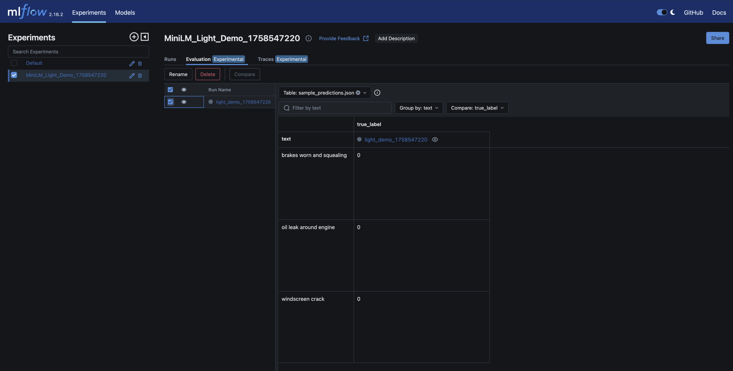
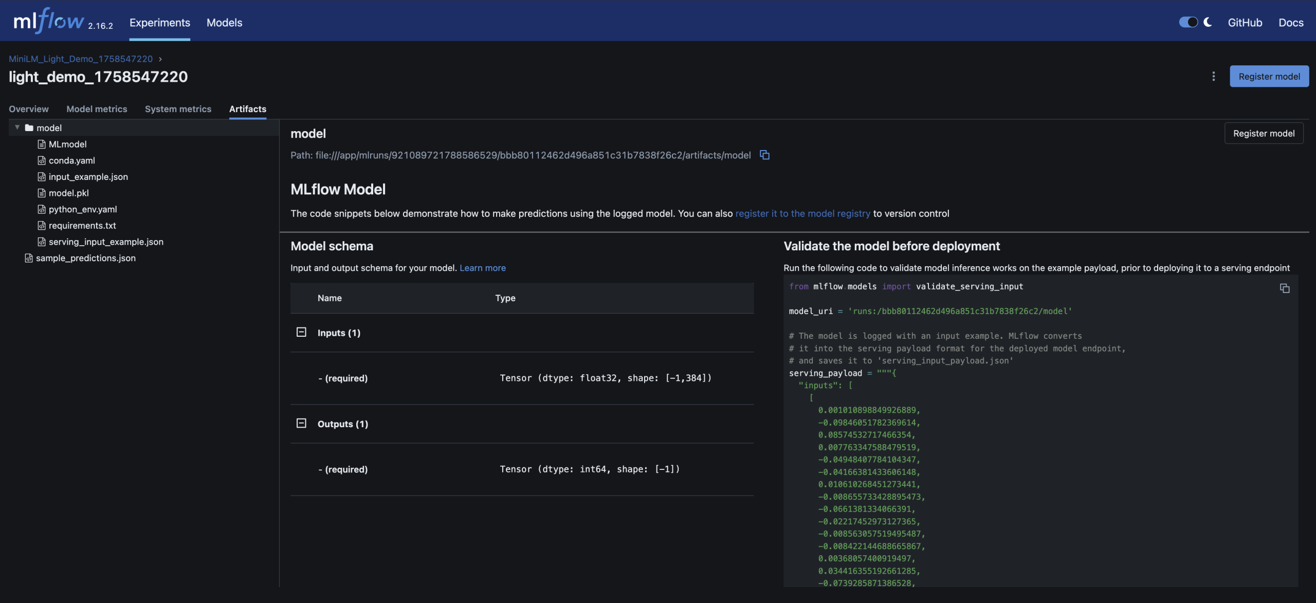
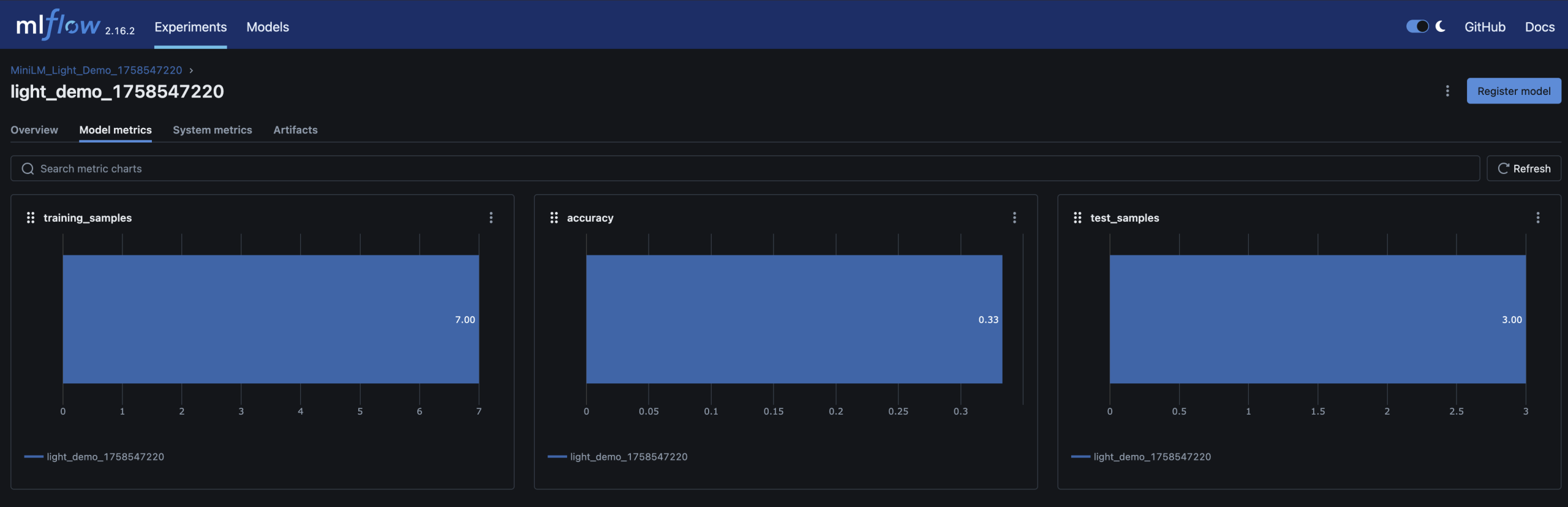
About the Author: This article was written as part of building Remora, a production-grade market risk engine for algorithmic trading systems. The system is built using modern Python async frameworks (FastAPI), time-series databases (ClickHouse), and MLOps best practices for real-time data aggregation and risk assessment.
Have questions about integrating Remora with Freqtrade? Found this useful? I’d love to hear your feedback or see your integration examples. Feel free to reach out or share your experiences.